On Instabilities of Conventional Multi-Coil MRI Reconstruction To Small Adversarial Perturbations
Chi Zhang1,2, Jinghan Jia3, Burhaneddin Yaman1,2, Steen Moeller2, Sijia Liu4, Mingyi Hong1, and Mehmet Akçakaya1,2 1Electrical and Computer Engineering, University of Minnesota, Minneapolis, MN, United States, 2Center for Magnetic Resonance Research, University of Minnesota, Minneapolis, MN, United States, 3University of Florida, Gainesville, FL, United States, 4MIT-IBM Watson AI Lab, IBM Research, Cambridge, MA, United States
Conventional multi-coil
reconstructions are also susceptible to large instabilities from small
adversarial perturbations. It
is worthwhile to interpret the instabilities of DL methods within this broader
context for the practical multi-coil setting.
Figure
2. Reconstruction results for uniform undersampling without (top row) and with (bottom row)
attack. The small perturbation causes no visual difference in the fully-sampled
image or the zero-filled image. The reconstructions without attack show some
residual aliasing due to the R=4 acceleration. Both CG-SENSE and GRAPPA visibly
fail with the small perturbation attack.
Figure
3. Reconstruction results for
random undersampling without (top row) and with (bottom row) attack. The small
perturbation leads to no visual change in the fully-sampled or zero-filled
image. For the input without attack, CG-SENSE has visible and multi-coil CS has
subtle aliasing artifacts at R=4. For the attack input, both these
reconstructions fail although they are run with the exact same parameters as
the non-attack case.
Subtle Inverse Crimes: Naively using Publicly Available Images Could Make Reconstruction Results Seem Misleadingly Better!
Efrat Shimron1, Jonathan Tamir2, Ke Wang1, and Michael Lustig1 1Electrical Engineering and Computer Sciences, UC Berkeley, Berkeley, CA, United States, 2Electrical and Computer Engineering, The University of Texas at Austin, Austin, TX, United States
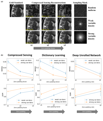
This work reveals that naïve training and evaluation of reconstruction algorithms on publicly available data could lead to artificially improved reconstructions. We demonstrate that Compressed Sensing, Dictionary Learning and Deep Learning algorithms may all produce misleading results.
Subtle Crime I Results. (a) CS reconstructions from data subsampled with R=6. The subtle crime effect is demonstrated: the reconstruction quality improves artificially as the sampling becomes denser around k-space center (top to bottom) and the zero-padding increases (left to right). (b) The same effect is shown for CS (mean & STD of 30 images), Dictionary Learning (10 images), and DNN algorithms (87 images): the NRMSE and SSIM improve artificially with the zero-padding and sampling.
Subtle Crime II concept. MR images are often saved in the DICOM format which sometimes involves JPEG compression. However, JPEG-compressed images contain less high-frequency data than the original data; therefore, algorithms trained on retrospectively-subsampled compressed data may benefit from the compression. These algorithms may hence exhibit misleadingly good performance.
Motion-resolved B1+ prediction using deep learning for real-time pTx pulse-design.
Alix Plumley1, Luke Watkins1, Kevin Murphy1, and Emre Kopanoglu1 1Cardiff University Brain Research Imaging Centre, Cardiff, United Kingdom
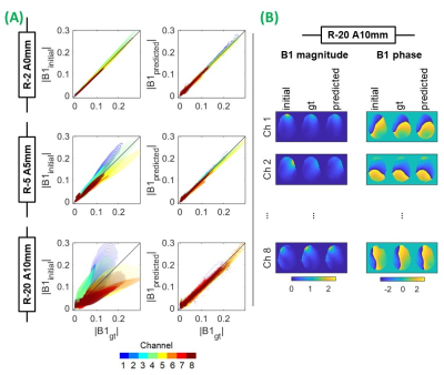
We present a deep learning approach to estimate motion-resolved parallel-transmit B1+ distributions using a system of conditional generative adversarial networks. The estimated maps can be used for real-time pulse re-design, eliminating motion-related flip-angle error.
Fig.4(A) Voxelwise magnitude
correlations between B1initial (initial position) and B1gt (ground-truth
displaced) [left] and B1predicted (network predicted displaced) and
B1gt [right]. Small (top), medium (middle) and large (bottom) displacements are shown. Phase data not shown. (B) Magnitude
(in a.u.) and phase (radians) B1-maps for the largest displacement.
Left, middle and right: B1initial, B1gt and
B1predicted, respectively. B1predicted
quality did not depend heavily on displacement magnitude and remained high
despite 5 network cascades for evaluation at R-20 A10mm.
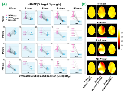
Fig.3(A) Motion-induced
flip-angle error for pTx pulses designed using B1initial
(conventional method, pink) & B1predicted (proposed method,
blue) at all evaluated positions & slices. Y-axes show nRMSE (% target
flip-angle). nRMSE of all pulsespredicted is at/below the shaded
region. Asterisks show number of network cascades required for evaluation. (B) Example profiles. Left: evaluation for pulseinitial
without motion. Middle & right: evaluations at
B1gt (displaced position) using pulseinitial & pulsepredicted,
respectively. Colorscale shows flip-angle (target=70°).
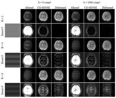
Robust Multi-shot EPI with Untrained Artificial Neural Networks: Unsupervised Scan-specific Deep Learning for Blip Up-Down Acquisition (BUDA)
Tae Hyung Kim1,2,3, Zijing Zhang1,2,4, Jaejin Cho1,2, Borjan Gagoski2,5, Justin Haldar3, and Berkin Bilgic1,2 1Athinoula A. Martinos Center for Biomedical Imaging, Boston, MA, United States, 2Radiology, Harvard Medical School, Boston, MA, United States, 3Electrical Engineering, University of Southern California, Los Angeles, CA, United States, 4State Key Laboratory of Modern Optical Instrumentation, College of Optical Science and Engineering, Zhejiang University, Hangzhou, China, 5Boston Children's Hospital, Boston, MA, United States
A novel unsupervised, untrained, scan-specific artificial neural network from LORAKI framework for blip-up and down acquisition (BUDA) enables robust reconstruction of multi-shot EPI.
Figure 1. The structure of the proposed network. “A” represents the BUDA forward model, “B” is SENSE-encoding (coil sensitivities and Fourier transform), “VC” represents augmentation of virtual conjugate coils for the phase constraint. Some parameter choices are: the number of iteration K=7, convolution kernel size=7, The number of output channels of the first convolutional layer=64, λ1 = 1, λ2 = 0.5.
Figure 2. The reconstruction results of the diffusion data with b=1000s/mm2 . Top two rows display reconstructed images, the bottom two rows show error images (10x-amplified). For each shot, 4x in-plane acceleration was applied. Two shots (one blip-up and one blip-down) were used for reconstruction. The reference images were generated by combining 4 shots (2 blip-up and 2 blip-down) through BUDA. Naive SENSE does not include the fieldmap, resulting in distortion near frontal lobes.
Deep
Low-rank plus Sparse Network for Dynamic MR Imaging
Wenqi Huang1,2, Ziwen Ke1,2, Zhuo-Xu Cui1, Jing Cheng2,3, Zhilang Qiu2,3, Sen Jia3, Yanjie Zhu3, and Dong Liang1,3 1Research Center for Medical AI, Shenzhen Institutes of Advanced Technology, Chinese Academy of Sciences, Shenzhen, China, 2Shenzhen College of Advanced Technology, University of Chinese Academy of Sciences, Shenzhen, China, 3Paul C. Lauterbur Research Center for Biomedical Imaging, Shenzhen Institutes of Advanced Technology, Chinese Academy of Sciences, Shenzhen, China
We propose a model-based low-rank plus
sparse network (L+S-Net) for dynamic MR reconstruction. A learned singular
value thresholding was introduced to explore the deep low rank prior. Experiment
results show that it can improve the reconstruction both qualitatively and
quantitatively.
Fig. 1. The proposed sparse plus low-rank network
(L+S-Net) for dynamic MRI. The L+S-Net is defined by the iterative procedures
of Eq.(5). The three layers correspond to the three modules in L+S-Net, which
are named as low-rank prior layer, sparse prior layer and data consistency layer respectively. The convolution block in sparse prior layer is shown at the left bottom. The correction
term in data consistency layer is shown at the right bottom.
Fig. 3. The reconstruction results of the
different methods (L+S, MoDL and L+S-Net) at 12-fold acceleration using
multi-coil data. The first row shows, from left to right, the ground truth, the
reconstruction result of these methods. The second row shows the enlarged view
of their respective heart regions framed by a yellow box. The third row shows
the error map (display ranges [0, 0.07]). The y-t image (extraction of the 92th
slice along the y and temporal dimensions) and the error of y-t image are also
given for each signal to show the reconstruction performance in the temporal
dimension.
Joint Reconstruction of MR Image and Coil Sensitivity Maps using Deep Model-based Network
Yohan Jun1, Hyungseob Shin1, Taejoon Eo1, and Dosik Hwang1 1Electrical and Electronic Engineering, Yonsei University, Seoul, Korea, Republic of
We propose a Joint
Deep Model-based MR Image and Coil Sensitivity Reconstruction Network (Joint-ICNet),
which jointly reconstructs an MR image and coil sensitivity maps from
undersampled multi-coil k-space data using deep learning networks combined with
MR physical models.
Fig. 1. Overall framework of our proposed joint deep model-based
magnetic resonance image and coil sensitivity reconstruction network
(Joint-ICNet).
Fig. 3. Fully sampled and reconstructed (a) FLAIR images and (b) T2 images using
zero-filling, ESPIRiT, U-net, k-space learning, DeepCascade, and Joint-ICNet,
with the reduction factors R = 4 and R =8, respectively.
Ungated time-resolved cardiac MRI with temporal subspace constraint using SSA-FARY SE
Sebastian Rosenzweig1,2 and Martin Uecker1,2 1Diagnostic and Interventional Radiology, University Medical Center Göttingen, Göttingen, Germany, 2Partner Site Göttingen, German Centre for Cardiovascular Research (DZHK), Göttingen, Germany
SSA-FARY SE is a simple yet powerful novel method to estimate a suitable temporal basis for subspace reconstructions of time-series data from a potentially very small auto-calibration region.
FIG_2: Comparison of the single-slice temporal subspace reconstruction with a rank $$$N_\text{b}=30$$$ subspace estimated using PCA (left) and SSA-FARY SE (right). The movie shows a 1.8s snippet of the full time-series. The snippet corresponds to the time-frames highlighted by the orange box in FIG_3. (The movie of the full time-series could not be included here due to file-size limits.)
FIG_4: Real- and imaginary part of the six most significant temporal basis functions $$$T\,1\;-\;T\,6$$$ and the corresponding complex image coefficients for PCA (left) and SSA-FARY SE (right). The temporal basis functions are provided by the columns of the matrix $$$U$$$, see Step 2 of the theory section.
A unified model for simultaneous reconstruction and R2* mapping of accelerated 7T data using the Recurrent Inference Machine
Chaoping Zhang1, Dirk Poot2, Bram Coolen1, Hugo Vrenken3, Pierre-Louis Bazin4,5, Birte Forstmann4, and Matthan W.A. Caan1 1Biomedical Engineering & Physics, Amsterdam UMC, Amsterdam, Netherlands, 2Biomedical Imaging Group Rotterdam, Erasmus MC, Rotterdam, Netherlands, 3Radiology, Amsterdam UMC, Amsterdam, Netherlands, 4Integrative Model-based Cognitive Neuroscience research unit, University of Amsterdam, Amsterdam, Netherlands, 5Max Planck Institute for Human Cognitive and Brain Sciences, Leipzig, Germany
We present a unified model embedded in the Recurrent Inference Machine for joint reconstruction and estimation of R2*-maps from subsampled k-space data. Applied to a cohort study, this leads to an improved reconstruction and estimation,increasingly improving for higher acceleration
Left: The quantitative
Recurrent Inference Machine jointly reconstructs and estimates an R2*-map from
sparsely sampled multi-echo gradient echo data. Right: The netwerk architecture
of the quantitative Recurrent Inference Machine is shown with the log-likelihood
function l(M,R2*,B0) depicted on top.
Example R2* images of the
reference image and 12-times accelerated reconstructions using the RIM with
least-squares fit, and the proposed method qRIM with integrated reconstruction
and parameter estimation.
Joint Data Driven Optimization of MRI Data Sampling and Reconstruction via Variational Information Maximization
Cagan Alkan1, Morteza Mardani1, Shreyas S. Vasanawala1, and John M. Pauly1 1Stanford University, Stanford, CA, United States
Variational information maximization enables end-to-end optimization of MR data sampling and reconstruction in a data-driven manner. Our framework improves the reconstruction quality as measured by the 1.4-2.2dB increase in pSNR compared to the variable density baseline.
Figure 4: Reconstruction result from a slice in the test set for $$$R=5$$$ and $$$R=10$$$. Zero-filled reconstruction corresponds to applying $$$A_\phi^H$$$ on $$$z$$$ directly.
Figure 1: Network architecture consisting of nuFFT based encoder (a) and unrolled reconstruction network (b, c). Sampling locations $$$\phi$$$ are shared between encoder and decoder.
Design of slice-selective RF pulses using deep learning
Felix Krüger1, Max Lutz1, Christoph Stefan Aigner1, and Sebastian Schmitter1 1Physikalisch-Technische Bundesanstalt, Braunschweig and Berlin, Germany
We utilize a residual neural network for the
design of slice selective RF and gradient trajectories. The network was trained
with 300k SLR RF pulses. It predicts the RF pulse and the gradient for a desired
magnetization profile. We evaluate the feasibility and limitations of this new
approach.
Figure 3: The NRMSE over the whole parameters space. In blue the results for the Network I trained
on 1D slice-selective SLR pulses for different validation data sets are shown.
In red the same principle was extended to Network II, for which SMS pulses were
included in the library. The first row ((a)-(c) displays the influence of the BWTP, the second row ((d)-(f)) with respect to the FA and the
third row ((g)-(i)) to a varying slice thickness
. The last row ((j)-(l)) shows the influence of
the slice shift
. The relations are evaluated for the
magnetization profile, the RF pulse and the gradient.
Figure 2: Representative example for a validation data set
with a BWTP of 7, FA of 45°, slice thickness of 7mm and no slice shift used on the
pretrained neural network is shown. In (e), (f), (g) the output is compared to the
ground truth. The prediction is used for a second Bloch simulation to analyze
the difference between the desired and the predicted magnetization in (a), (b), (c), (d). The predicted result is in good agreement with the ground truth for
this parameter set.
Adapting the U-net for Multi-coil MRI Reconstruction
Makarand Parigi1, Abhinav Saksena1, Nicole Seiberlich2, and Yun Jiang2 1Computer Science and Engineering, University of Michigan, Ann Arbor, MI, United States, 2Department of Radiology, University of Michigan, Ann Arbor, MI, United States
Applying a neural network before and after the coil combination step of MRI reconstruction produces higher quality images with lower memory usage.
Figure 1: Illustration of the Multinet architecture, featuring the Multi-image U-net and a traditional U-net. The Multi-image U-net takes in as many images as there are coils, and outputs that many images.
Figure 2: Illustration of the Multi-image U-net, the first component of the Multinet. The number in the boxes indicates the number of channels, while the width and height of the data is displayed to the side. x is the number of channels in the output of the first convolution, i.e. Multinet-16 would have x=16. n is the number of input and output channels of the entire model. For the Multinet, this is the number of coils.
Multi-channel and multi-group-based CNN Image Reconstruction using Equal-sized Multi-resolution Image Decomposition
Shohei Ouchi1 and Satoshi ITO1 1Utsunomiya University, Utsunomiya, Japan
The
transformed image domain CNN-CS method were proposed based on the equal-sized
multi-resolution image decomposition method. Reconstruction experiments showed
this CNN-CS could reconstruct sharp images that have strong phase variation.
Fig.5 Comparison of reconstructed images between eFREBAS-CNN, Image Domain CNN, ADMM-CSNet and CS iterative. (h) – (m) are the enlarged images of (a) – (f), respectively.
Fig.3 Network architecture and reconstruction flow of eFREBAS-CNN. Three groups are reconstructed by three CNNs, respectively. U-Net2 and U-Net3 that treats Group B and Group C are input lower frequency sub-images as shown in Fig.2.
Rethinking complex image reconstruction: ⟂-loss for improved complex image reconstruction with deep learning
Maarten Terpstra1,2, Matteo Maspero1,2, Jan Lagendijk1, and Cornelis A.T. van den Berg1,2 1Department of Radiotherapy, University Medical Center Utrecht, Utrecht, Netherlands, 2Computational Imaging Group for MR diagnostics & therapy, University Medical Center Utrecht, Utrecht, Netherlands
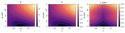
The \(\ell^2\) norm is the default loss function for complex image reconstruction. In this work, we identify unexpected behavior for \(\ell^p\) loss functions, propose a new loss function, which improves deep learning complex image reconstruction performance.
Figure 2: Simulation of loss landscapes. The loss landscapes of the \(\ell^1, \ell^2,\) and \(\perp\)-loss are shown, respectively. For every \((\phi, \lambda)\) pair, \(10^5\) random complex number pairs were generated. Contours show lines of equal loss. The figures show that \(\perp\)-loss is symmetric around \(\lambda\), whereas the \(\ell^1\) and \(\ell^2\) loss functions have a higher loss for \(\lambda > 1\).
Figure 3: Typical reconstructions. Typical magnitude reconstructions from the \(\ell^1\), \(\ell^2\) and \(\perp\)-loss networks with R=5. Top row shows magnitude target and reconstructions, with respective squared error maps below. The training with our loss function reconstructs smaller details as highlighted by the red arrows. Third row shows phase map target and reconstructions, with respective error maps below. Significant phase artifacts not present in \(\perp\)-loss are highlighted.
PCA and U-Net based Channel Compression for Fast MR Image Reconstruction
Madiha Arshad1, Mahmood Qureshi1, Omair Inam1, and Hammad Omer1 1Medical Image Processing Research Group (MIPRG), Department of Electrical and Computer Engineering, COMSATS University, Islamabad, Pakistan
The
proposed method retains the virtual coil sensitivity information better as
compared to that of PCA. Moreover, the proposed channel compression reduces the
size of the input data with minimum channel compression losses before
reconstruction.
Figure 1: Block diagram of the proposed method: First, PCA is applied to
compress the VD under-sampled human head data from 30 channel receiver coils to
8 virtual coils. Later U-Net is used to compensate the compression losses of
PCA in terms of sensitivity information of 8 virtual coils VD under-sampled
images. Later, adaptive coil combination of CS-MRI reconstructed virtual coil
images gives the final solution/reconstructed image.
Figure 2: CS-MRI reconstructed 8 virtual coil images obtained from the proposed
channel compression and PCA: First the VD under-sampled human head data (AF=2)
is compressed from 30 channel receiver coils into 8 virtual coils by the proposed
method and PCA. Later, CS-MRI is used for coil-by-coil reconstruction of 8
virtual coil under-sampled images. The reconstructed virtual coil images show
minimum compression losses by the proposed method as compared to the PCA.
Moritz Blumenthal1 and Martin Uecker1,2,3,4 1Institute for Diagnostic and Interventional Radiology, University Medical Center Göttingen, Göttingen, Germany, 2DZHK (German Centre for Cardiovascular Research), Göttingen, Germany, 3Campus Institute Data Science (CIDAS), University of Göttingen, Göttingen, Germany, 4Cluster of Excellence “Multiscale Bioimaging: from Molecular Machines to Networks of Excitable Cells” (MBExC), University of Göttingen, Göttingen, Germany
By integrating deep learning into BART, we have created a reliable framework combining state-of-the-art MRI reconstruction methods with neural networks. For MoDL and the Variational Network, we achieve similar performance as implementations using TensorFlow.
Figure 2: Nlops and automatic differentiation. a) A basic nlop modeled by the operator $$$F$$$ and derivatives $$$\mathrm{D}F$$$. When applied, $$$F$$$ stores data internally such that the $$$\mathrm{D}F$$$s are evaluated at $$$F$$$'s last inputs. b) Chaining two nlops $$$F$$$ and $$$G$$$ automatically chains their derivatives obeying the chain rule. The adjoint of the derivative can be used to compute the gradient by backpropagation. c) Composition of a residual structure $$$F(\mathbf{x}, G(\mathbf{x},\mathbf{y}))$$$ by combine, link and duplicate.
Figure 1: Basic structure of the BART-libraries used for deep learning: Networks are implemented as nlops supporting automatic differentiation. The nn-library provides deep-learning specific components such as initializers. Training algorithms have been integrated BART's library for iterative algorithms. MD-functions act as a flexible, unified interface to the numerical backend. We added many deep-learning specific nlops such as convolutions using efficient numerical implementations. Solid blocks represent major changes allowing deep learning.
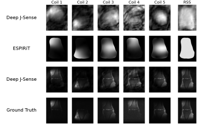
Deep J-Sense: An unrolled network for jointly estimating the image and sensitivity maps
Marius Arvinte1, Sriram Vishwanath1, Ahmed H Tewfik1, and Jonathan I Tamir1,2,3 1Electrical and Computer Engineering, The University of Texas at Austin, Austin, TX, United States, 2Diagnostic Medicine, Dell Medical School, The University of Texas at Austin, Austin, TX, United States, 3Oden Institute for Computational Engineering and Sciences, The University of Texas at Austin, Austin, TX, United States
We introduce a deep learning-based accelerated MRI reconstruction method that unrolls an alternating optimization and jointly estimates the image and coil sensitivity maps. We show competitive results against state-of-the-art methods and faster convergence in poor channel conditions.
Block diagram of the
approach. (a) Inside each unrolling step, the pair of variables is updated in
an alternating fashion with M steps of CG applied to each variable. The red
blocks represent the learnable parameters of Deep J-Sense and are shared across
unrolls. The numbers in parentheses corresponding to the four update steps in
the text. (b) N unrolls are applied starting from initial values. At each step,
the gradient of the loss term is back-propagated to the trainable parameters and
an update is performed.
Examples of estimated
sensitivity maps and reconstructed coil images output by our method after N = 6
unrolls for a validation sample with R = 4. The first five columns show specific
coils and the last columns shows the RSS image obtained from all 15 coils. The
first row shows the estimated sensitivity maps, obtained by zero-padding and
IFFT of the estimated frequency-domain kernel. The second row shows the
sensitivity maps estimated using the auto-ESPIRiT algorithm. The
third row shows the reconstructed coil images.
The fourth row shows the ground truth (fully-sampled) coil images.
Using data-driven image priors for image reconstruction with BART
Guanxiong Luo1, Moritz Blumenthal1, and Martin Uecker1,2 1Institute for Diagnostic and Interventional Radiology, University Medical Center Göttingen, Germany, Göttingen, Germany, 2Campus Institute Data Science (CIDAS), University of Göttingen, Germany, Göttingen, Germany
The application of deep learning has is a new paradigm for MR image reconstruction. Here, we demonstrate how to incorporate trained neural networks into pipelines using reconstruction operators already provided by the BART toolbox.
Figure 1. The python program to train a generic prior consists of components illustrated above.
Figure 3. Reconstructions from 60 radial k-space spokes via zero-filled, iterative sense, $$$\ell_1$$$-wavelet, learned log-likelihood (left to right).
Going beyond the image space: undersampled MRI reconstruction directly in the k-space using a complex valued residual neural network
Soumick Chatterjee1,2,3, Chompunuch Sarasaen1,4, Alessandro Sciarra1,5, Mario Breitkopf1, Steffen Oeltze-Jafra5,6,7, Andreas Nürnberger2,3,7, and Oliver Speck1,6,7,8 1Department of Biomedical Magnetic Resonance, Otto von Guericke University, Magdeburg, Germany, 2Data and Knowledge Engineering Group, Otto von Guericke University, Magdeburg, Germany, 3Faculty of Computer Science, Otto von Guericke University, Magdeburg, Germany, 4Institute of Medical Engineering, Otto von Guericke University, Magdeburg, Germany, 5MedDigit, Department of Neurology, Medical Faculty, University Hopspital, Magdeburg, Germany, 6German Centre for Neurodegenerative Diseases, Magdeburg, Germany, 7Center for Behavioral Brain Sciences, Magdeburg, Germany, 8Leibniz Institute for Neurobiology, Magdeburg, Germany
The preliminary experiments with fastMRI dataset have
shown promising results. The network was able to reconstruct undersampled MRIs
with less to no artefact, and resulted in SSIM as high as 0.955, improving from
0.877.
Fig.2: Reconstruction result of the random variable density sampling, along with the fully-sampled image, undersampled (zero-padded) image and the corresponding difference images.
Fig.1. Network architecture and the workflow of the proposed complex valued residual neural network. The network is provided with undersampled k-space for each coil, treating each coil as different channel. The network also provided coil-wise k-space as output. The originally acquired data were then replaced in the output k-space as a data consistency step. 2D inverse fast Fourier transform (IFFT) was performed on this k-space to obtain the coil-wise reconstructed images. IFFT was also performed on the fully sampled k-space and then the loss was computed by comparing these images.
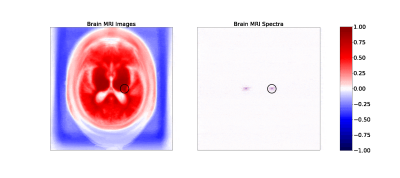
A Deep-Learning Framework for Image Reconstruction of Undersampled and Motion-Corrupted k-space Data
Nalini M Singh1,2, Juan Eugenio Iglesias1,3,4, Elfar Adalsteinsson2,5,6, Adrian V Dalca1,4, and Polina Golland1,5,6 1Computer Science and Artificial Intelligence Laboratory, Massachusetts Institute of Technology, Cambridge, MA, United States, 2Harvard-MIT Division of Health Sciences and Technology, Massachusetts Institute of Technology, Cambridge, MA, United States, 3Centre for Medical Image Computing, University College London, London, United Kingdom, 4A. A. Martinos Center for Biomedical Imaging, Department of Radiology, Massachusetts General Hospital, Charlestown, MA, United States, 5Department of Electrical Engineering and Computer Science, Massachusetts Institute of Technology, Cambridge, MA, United States, 6Institute for Medical Engineering and Science, Massachusetts Institute of Technology, Cambridge, MA, United States
We demonstrate high quality image reconstruction of undersampled k-space data corrupted by significant motion. Our deep learning approach exploits correlations in both frequency and image space and outperforms frequency and image space baselines.
Figure 4. Top: Example reconstructions with motion induced at 3% of scanning lines. The Interleaved and Alternating architectures more accurately eliminate the 'shadow' of the moved brain and the induced ringing and blurring compared to the single-space networks.
Bottom: Comparison of all four network architectures on test samples with motion at varying fractions of lines. For nearly every example, the joint architectures (Interleaved and Alternating) outperform the single-space baselines.
Figure 1. Maps of correlation coefficients between a single pixel (circled) and all other pixels in image (left) and frequency (right) space representations of the brain MRI dataset (click to view an animation of correlation patterns at several pixels). Both maps show strong local correlations useful for inferring missing or corrupted data. Frequency space correlations also display conjugate symmetry characteristic of Fourier transforms of real images.
DeepSlider: Deep learning-powered gSlider for improved robustness and performance
Juhyung Park1, Dongmyung Shin1, Hyeong-Geol Shin1, Jiye Kim1, and Jongho Lee1 1Seoul National University, Seoul, Korea, Republic of
Slab-encoding RF pulses are designed
using deep reinforcement learning to optimize the condition number of the RF
encoding matrix. The newly designed RF pulses show improved robustness and
performance compared to conventional gSlider designs.
Figure 1. Overview of DeepSlider. Five
slab-encoding RF pulses are designed using deep reinforcement learning and
gradient descent. The signals
from slab-encoding RF pulses can be modeled as
a linear system of an encoding matrix
and sub-slice signals z. The design objective is
to minimize the condition number of the encoding matrix A, improving stability
against noise.
Figure 2. Details of generating
slab-encoding RF pulses. (a) In a single episode, DRL agent generates an RF
pulse as an action, and Bloch equation
environment returns a reward for the RF pulse. The reward is composed of slice
profile penalty and SAR regularization. The agent is updated using the reward
and generates an RF pulse recursively to maximize the reward. (b) DRL-generated
RF pulses are randomly grouped into five RF pulses. Then the five RF pulses are
optimized to have the lowest condition number in the encoding matrix
(and maximize DRL reward term) by gradient
descent.
Intelligent Incorporation of AI with Model Constraints for MRI Acceleration
Renkuan Zhai1, Xiaoqian Huang2, Yawei Zhao1, Meiling Ji1, Xuyang Lv2, Mengyao Qian1, Shu Liao2, and Guobin Li1 1United Imaging Healthcare, Shanghai, China, 2United Imaging Intelligence, Shanghai, China
AI-assisted Compressed Sensing is introduced to realize superior MR acceleration and address the uncertainty of CNN by incorporating the output
of AI as one more regularization term.
Figure 1. ACS flowchart: AI Module represents
the trained AI network; CS Module is for solving the second formula using iterative
reconstruction.
Figure 2. T2 FSE 2D of knee with acceleration factors from 2.00x to 4.00x.
As acceleration factor increased, quality of CS images degraded more rapidly than
ACS.
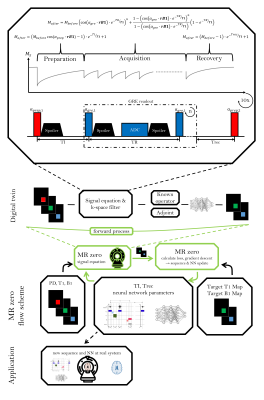
MRzero sequence generation using analytic signal equations as forward model and neural network reconstruction for efficient auto-encoding
Simon Weinmüller1, Hoai Nam Dang1, Alexander Loktyushin2,3, Felix Glang2, Arnd Doerfler1, Andreas Maier4, Bernhard Schölkopf3, Klaus Scheffler2,5, and Moritz Zaiss1,2 1Neuroradiology, University Clinic Erlangen, Friedrich-Alexander Universität Erlangen-Nürnberg (FAU), Erlangen, Germany, 2Max-Planck Institute for Biological Cybernetics, Magnetic Resonance Center, Tübingen, Germany, 3Max-Planck Institute for Intelligent Systems, Empirical Inference, Tübingen, Germany, 4Pattern Recognition Lab Friedrich-Alexander-University Erlangen-Nürnberg, Erlangen, Germany, 5Department of Biomedical Magnetic Resonance, Eberhard Karls University Tübingen, Tübingen, Germany
Using analytic
signal equations combined with neural network reconstruction allows fast, fully
differentiable supervised learning of MRI sequences. This forms a fast
alternative to the full Bloch-equation-based MRzero framework in certain cases.
Figure 1: Schematic
of the MRzero framework. Topmost part: An MR image is simulated for given
sequence parameters and Bloch parameters (PD, B1 and T1) with an analytic signal equation. The evolution of the signals
are mapped pixelwise to B1 and T1 values with a NN. The output is compared to
the target (B1 and T1 value) and gradient descent optimization is performed to update sequence
parameters TI, Trec, TR, $$$\alpha_{gre}$$$, $$$\alpha_{prep}$$$ and NN parameters.
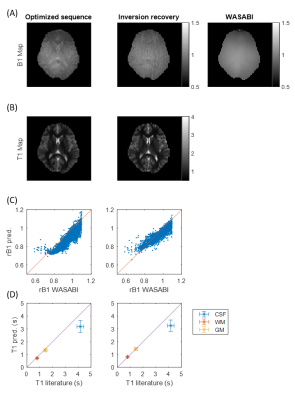
Figure 4: Pixelwise evaluation
of the NN-predicted B1 (A) and T1 (B) maps for the optimized sequence (first column)
and the inversion recovery (second column). B1 map from the WASABI measurement
as reference (third column). Correlation between
WASABI and optimized sequence with correlation coefficient R=0.88 and
correlation between WASABI and inversion recovery with correlation coefficient
R=0.90 (C). Comparison of obtained T1 values for different tissue ROIs with
literature values (D).
AutoSON: Automated Sequence Optimization by joint training with a Neural network
Hongjun An1, Dongmyung Shin1, Hyeong-Geol Shin1, Woojin Jung1, and Jongho Lee1 1Department of Electrical and computer Engineering, Seoul National University, Seoul, Korea, Republic of
A new optimization method for MRI sequences is proposed. This method jointly optimizes the sequence and a neural estimator that extracts information (e.g. quantitative mapping ) from MR signals. The method shows well-optimized results regardless of problems.
Figure
1. Overview
of AutoSON. (a) Structure of AutoSON. AutoSON contains an MRI simulator for the
generation of training signals and a neural network that extracts target information
for the objective. (b) Joint optimization of AutoSON. The distribution of tissue
properties and noise conditions were utilized to generate training data. Using
this data, joint optimization was performed for scan parameters and weights of
the neural network using a loss function for the objective. (c) After the joint
optimization, the sequence parameters were optimized for the objective.
Figure
4. Partially
spoiled SSFP T2 mapping results of the scan parameters. The AutoSON optimized
parameters yielded better performance than the parameters from Wang et al. in
a computer simulation, although the mapping was
performed by without a neural network.
Deep Learning Based Joint MR Image Reconstruction and Under-sampling Pattern Optimization
Vihang Agarwal1, Yue Cao1, and James Balter1 1Radiation Oncology, University of Michigan, Ann Arbor, MI, United States
We demonstrate joint optimization of under-sampling patterns with the proposed image reconstruction neural network architecture allows under-sampling with higher acceleration rates and produces superior quality images as compared to random under-sampling schemes.
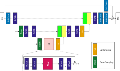
The architecture of our Attentive Residual Non Local-Network (ARNL-Net) with RCAB as building blocks.
Image reconstructions under cartesian constrained acquisition scheme. Second row demonstrates the results for the joint optimization model.
ArtifactID: identifying artifacts in low field MRI using deep learning
Marina Manso Jimeno1,2, Keerthi Sravan Ravi2,3, John Thomas Vaughan Jr.2,3, Dotun Oyekunle4, Godwin Ogbole4, and Sairam Geethanath2 1Biomedical Engineering, Columbia University, New York, NY, United States, 2Columbia Magnetic Resonance Research Center (CMRRC), New York, NY, United States, 3Columbia University, New York, NY, United States, 4Radiology, University College Hospital, Ibadan, Nigeria
ArtifactID utilizes deep learning to identify wrap-around and Gibbs ringing artifacts in 0.36T MR images. The models achieved accuracies of 88% and 89.5%, respectively. Wrap-around filter visualization confirms learning of the identified artifact.
Figure 1. Artifacts simulated in this work and identified in the low-field dataset. a) Representative input brain slice (b-e) Gibbs ringing and wrap-around artifacts simulated in this work b) Gibbs ringing artifact c) X-axis wrap-around artifact d) Y-axis wrap-around artifact e) Z-axis wrap-around artifact (f-i) Wrap-around artifacts identified in the low-field dataset (j-m) Gibbs ringing artifact identified in the low-field dataset.
Figure 4. Performance evaluation and model explanation via filter visualization for wrap-around artifact identification. (a) Confusion matrix obtained from the validation and test sets; in the case of simulated data, forward modeling parameters were tweaked based on the validation set results to improve performance. (b) Visualization of representative filters for a true-positive (TP), true-negative (TN), false-positive (FP) and a false-negative (FN) input for explainability.
Artificial Intelligence based smart MRI: Towards development of automated workflow for reduction of repeat and reject of scans
Raghu Prasad, PhD1, Harikrishna Rai, PhD1, and Sanket Mali1 1GE Healthcare, Bangalore, India
AI based
computer vision solution is developed to correct positioning errors through identification
of RF coil and anatomy of the patient using a 3D depth camera. We have done feasibility
study on the effects of EMI on camera data and have evaluated the impact of
camera on magnetic in-homogeneity.
Uncertainty estimation for DL-based motion artifact correction in 3D brain MRI
Karsten Sommer1, Jochen Keupp1, Christophe Schuelke1, Oliver Lips1, and Tim Nielsen1 1Philips Research, Hamburg, Germany
An uncertainty metric based on test-time augmentation is explored for 3D
motion artifact correction. Analysis on test data revealed that this metric
could accurately predict global error levels but failed in certain cases to
detect local “hallucinations”.
Example results from the synthetic test dataset
where the uncertainty metric Δy accurately predicted the validity of the
corrections: For the input image shown in the top row, the network produces a
faithful reconstruction of the ground truth image, which is accurately
predicted by the low uncertainty metric. For the center and bottom row,
substantial deviations from the ground truth can be observed (marked by
arrows), which is accurately predicted by the relatively high uncertainty
metric (SD=standard deviation).
Example results on the synthetic test dataset
where the uncertainty metric Δy did not accurately
predict the validity of the corrections. In particular, multiple local
hallucinations can be observed (indicated by red arrows), although the TTA
metric values are relatively low (Δy=0.3).
A 3D-UNET for Gibbs artifact removal from quantitative susceptibility maps
Iyad Ba Gari1, Shruti P. Gadewar1, Xingyu Wei1, Piyush Maiti1, Joshua Boyd1, and Neda Jahanshad1 1Imaging Genetics Center, Mark and Mary Stevens Neuroimaging and Informatics Institute, Keck School of Medicine of USC, Los Angeles, CA, United States
Gibbs ringing artifact remains a challenge in SWI studies. Here we propose a deep learning approach, which removes Gibbs artifacts while still preserving anatomical features. Our model’s results outperform current artifact removal methods.
QSM Pipeline: Raw phase and magnitude images from SWI are combined (Bernstein method), the phase is unwrapped (fast phase unwrapping algorithm), background removed (Laplacian boundary value method), and the QSM reconstructed (MEDI).
Comparison of de-Gibbs-ed outputs from MRtrix3 and our UNet model removing the simulated Gibbs artifacts that were generated by truncating 70% of the high frequency k-space components of a full-sized mask from an image with minimal visually detectable Gibbs artifact. The second row is a zoomed in look into the black square on the first row.
Extending Scan-specific Artifact Reduction in K-space (SPARK) to Advanced Encoding and Reconstruction Schemes
Yamin Arefeen1, Onur Beker2, Heng Yu3, Elfar Adalsteinsson4,5,6, and Berkin Bilgic5,7,8 1Department of Electrical Engineering and Computer Science, Massachusetts Institute of Technology, Cambridge, MA, United States, 2Department of Computer and Communication Sciences, École Polytechnique Fédérale de Lausanne, Lausanne, Switzerland, 3Department of Automation, Tsinghua University, Beijing, China, 4Massachusetts Institute of Technology, Cambridge, MA, United States, 5Harvard-MIT Health Sciences and Technology, Cambridge, MA, United States, 6Institute for Medical Engineering and Science, Cambridge, MA, United States, 7Athinoula A. Martinos Center for Biomedical Imaging, Charlestown, MA, United States, 8Department of Radiology, Harvard Medical School, Boston, MA, United States
Spark, a scan-specific model for accelerated MRI reconstruction, is extended to advanced encoding and reconstruction schemes. We show improvement in 3D imaging with integrated and external calibration data, and in multiband, wave-encoded imaging.
Figure
3: Comparison between 4 x 3 accelerated, l2-regularized GRAPPA using 3D kernels
trained on a reference scan, and an acceleration matched SPARK acquisition
(un-regularized GRAPPA-input). SPARK measured the 30 x 30 undersampled
ACS region with 2 x 2 undersampling and the exterior of kspace with 4 x 3
undersampling in the phase encode and partition directions. SPARK
exploits the same reference scan used in GRAPPA to achieve improvement at the
representative slices.
Figure 4: Comparisons between sense, sense + SPARK, wave encoding, and wave + SPARK reconstructions on a simulated multiband 5, in-plane acceleration 2, acquisition. Wave was simulated with a maximum Gy/Gz gradient amplitude of 16 $$$\frac{mT}{m}$$$ and two cycles. Complex gaussian noise was added to all simulated data. SPARK provides qualitative and quantitative rmse improvement for both the sense and wave reconstructions. Wave + SPARK achieves the best results on both the total slice group and individual slices.
Improving Deep Learning MRI Super-Resolution for Quantitative Susceptibility Mapping
Antoine Moevus1,2, Mathieu Dehaes2,3,4, and Benjamin De Leener1,2,4 1Departement of Computer and Software Engineering, Polytechnique Montréal, Montréal, QC, Canada, 2Institute of Biomedical Engineering, University of Montreal, Montréal, QC, Canada, 3Department of Radiology, Radio-oncology, and Nuclear Medicine, Université de Montréal, Montréal, QC, Canada, 4Research Center, Ste-Justine Hospital University Centre, Montreal, QC, Canada
We explored the application of deep learning for superresolution on QSM data. We demonstrated the importance of training strategies for superresolution. We evaluated different loss functions for training neural networks on brain QSM data.
Figure 3 - Qualitative comparison of the models on a selected slice for the whole brain and two selected regions (green and blue boxes). The AHEAD reference is subject 005 slice 158. The ** represents the unoptimized cyclic LR WIMSE.
Table 1 - Comparison of models performance using the MSE and SSIM metrics. MSE: low score refers to high performance, SSIM: high score refers to high performance. Best performances are highlighted.
A Marriage of Subspace Modeling with Deep Learning to Enable High-Resolution Dynamic Deuterium MR Spectroscopic Imaging
Yudu Li1,2, Yibo Zhao1,2, Rong Guo1,2, Tao Wang3, Yi Zhang3, Mathew Chrostek4, Walter C. Low4, Xiao-Hong Zhu3, Wei Chen3, and Zhi-Pei Liang1,2 1Department of Electrical and Computer Engineering, University of Illinois at Urbana-Champaign, Urbana, IL, United States, 2Beckman Institute for Advanced Science and Technology, University of Illinois at Urbana-Champaign, Urbana, IL, United States, 3Center for Magnetic Resonance Research, University of Minnesota, Minneapolis, MN, United States, 4Department of Neurosurgery, University of Minnesota, Minneapolis, MN, United States
This
work presents a machine learning-based method for high-resolution dynamic
deuterium MR spectroscopic imaging. Experimental results
demonstrated the feasibility of obtaining spatially resolved metabolic changes at
an unprecedented resolution (~10 μL spatial, 105 sec temporal).
Figure
4. High-resolution dynamic DMRSI results of rat brain tumors. (a)-(b): Results obtained by the Fourier-based and proposed
imaging scheme, including time-dependent concentration maps (left panel), metabolic
time courses (middle panel), and time evolution of 2H-spectra (right panel); here, the metabolic time
courses and spectra are from voxels at the center of the red and yellow circles
within tumor and normal appearing tissues. (c): Differences in the dynamic changes of deuterated
Lac (left panel) and Glx (right panel) between tumor and normal-appearing
tissues.
Figure
3. In vivo
DMRSI results from one healthy rat brain, obtained by (a) conventional Fourier-based imaging scheme, and
(b) the proposed imaging scheme. On the left panels are concentration maps of deuterated Glc and Glx at five different time points after the infusion of deuterated glucose; in the middle panels are time courses of deuterated Glc, Glx and Lac at two representative voxels at the center of the red
and yellow circles located at the right- and left-hemispheric cortex,
respectively; on the right panel is the time evolution of 2H-spectra
at the same voxels.
Removing structured noise from dynamic arterial spin labeling images
Yanchen Guo1, Zongpai Zhang1, Shichun Chen1, Lijun Yin1, David C. Alsop2, and Weiying Dai1 1Department of Computer Science, State University of New York at Binghamton, Binghamton, NY, United States, 2Department of Radiology, Beth Israel Deaconess Medical Center & Harvard Medical School, Boston, MA, United States
The deep neural network (DNN) model, with the noise
structure learned and incorporated, demonstrates consistent improved
performance in removing the structured noise from the ASL functional images
compared to the DNN model without the explicitly incorporated noise structure.
Fig. 1. (a) network architecture of the DNN1. (b) network architecture of the DNN2. Each CNN layer contains convolution (Conv), Rectified Linear Units (ReLU), and batch normalization (BN). The size of each CNN layer is shown on the box. A kernel size of 3*3 is used for each convolution.
Fig. 3. An example of (a) ground-truth image, and (b) denoised image by the DNN1 model, (c) denoised image by the DNN2 model is shown.
Learn to Better Regularize in Constrained Reconstruction
Yue Guan1, Yudu Li2,3, Xi Peng4, Yao Li1, Yiping P. Du1, and Zhi-Pei Liang2 1Institute for Medical Imaging Technology, School of Biomedical Engineering, Shanghai Jiao Tong University, Shanghai, China, 2Department of Electrical and Computer Engineering, University of Illinois at Urbana-Champaign, Urbana, IL, United States, 3Beckman Institute for Advanced Science and Technology, University of Illinois at Urbana-Champaign, Urbana, IL, United States, 4Mayo Clinic, Rochester, MN, United States
This
paper presents a novel learning-based method for efficient selection of optimal
regularization parameters for constrained reconstruction. The proposed method
will enhance the speed, effectiveness and practical utility of constrained
reconstruction.
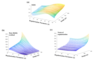
Figure
1. An
illustration of image quality manifolds for (a) SSIM, (b) data fidelity, and
(c) norm of regularization function. As can be seen, all image quality metrics,
as a function of
λ and ρ,
reside in a low-dimensional manifold and thus learnable from training data.
Figure
2. Comparison
of reconstruction results obtained from L-curve and the proposed method for
image deblurring. Note the reconstruction error was significantly reduced by
the proposed method, demonstrating its effectiveness in learning the optimal
regularization parameters.
Noise2Recon: A Semi-Supervised Framework for Joint MRI Reconstruction and Denoising using Limited Data
Arjun D Desai1,2, Batu M Ozturkler1, Christopher M Sandino3, Brian A Hargreaves2,3,4, John M Pauly3,5, and Akshay S Chaudhari2,5,6 1Electrical Engineering (Equal Contribution), Stanford University, Stanford, CA, United States, 2Radiology, Stanford University, Stanford, CA, United States, 3Electrical Engineering, Stanford University, Stanford, CA, United States, 4Bioengineering, Stanford University, Stanford, CA, United States, 5Equal Contribution, Stanford University, Stanford, CA, United States, 6Biomedical Data Science, Stanford University, Stanford, CA, United States
We propose Noise2Recon, a semi-supervised, deep-learning framework for accelerated MR reconstruction and denoising. Despite limited training data, Noise2Recon reconstructs both high and low-SNR scans with higher fidelity than supervised DL algorithms.
Fig. 1: Noise2Recon complements supervised training (blue pathway) with unsupervised training (red pathway) by enforcing network consistency between reconstructions of both unsupervised data and their noise-augmented counterparts. Unsupervised data is augmented by a noise map ε=U*F*N(0,σ), where σ is selected uniformly at random and the undersampling operator U is determined from the undersampled k-space. Scans with fully-sampled references follow the supervised training paradigm. The total loss is the weighted sum of the supervised (Lsup) and consistency (Lcons) losses.
Fig. 4: Reconstruction performance for 12x (top) and 16x (bottom) undersampled scans corrupted at varying noise levels (σ). Supervised models were trained with one (solid) or fourteen (dashed) supervised scans. Noise2Recon outperformed both 1-subject supervised methods at all noise levels. Noise2Recon achieved similar nRMSE and pSNR as noise-augmented supervised training but outperformed the latter in SSIM. Noise2Recon image quality metrics had low sensitivity to increasing σ and acceleration, which may indicate higher reconstruction robustness in noisy settings.
ENSURE: Ensemble Stein’s Unbiased Risk Estimator for Unsupervised Learning
Hemant Kumar Aggarwal1, Aniket Pramanik1, and Mathews Jacob1 1Electrical and Computer Engineering, University of Iowa, Iowa City, IA, United States
We proposed ENsample SURE loss function for MR image reconstruction problem using unsupervised learning. We show that training a network using an ensemble of images, each acquired with a different sampling pattern, can closely approximate the mean square error.
Fig. 3: ENSURE results on experimental data at 6-fold acceleration factor. Here we show the comparison of unsupervised training using the proposed ENSURE approach with supervised training as well as an existing unsupervised training approach SSDU [5]. The noise variance of the measurements was estimated, followed by the use of the SURE loss for training. The second row shows the zoomed cerebellum region. The third row shows error maps at 3x-scaling for visualization purposes. We observe that the ENSURE results closely match the MSE results with minimal blurring.
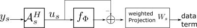
Fig. 1: The implementation details of the data-term in the proposed ENSURE approach for unsupervised training. First, we do the regridding reconstruction $$$\boldsymbol u_s$$$, then pass it through the network to get the reconstruction. Here the weighted projection term $$$\mathbf W_s$$$ represents the weighting of the k-space sample together with projection onto range space of $$$\mathcal A_s^H$$$. We note that this data-term does not require the ground truth image.
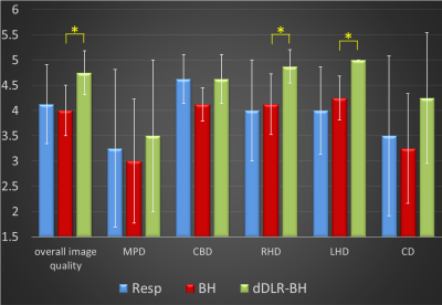
Breath-hold 3D MRCP at 1.5T using Fast 3D mode and a deep learning-based noise-reduction technique
Taku Tajima1,2, Hiroyuki Akai3, Koichiro Yasaka3, Rintaro Miyo1, Masaaki Akahane2, Naoki Yoshioka2, and Shigeru Kiryu2 1Department of Radiology, International University of Health and Welfare Mita Hospital, Tokyo, Japan, 2Department of Radiology, International University of Health and Welfare Narita Hospital, Chiba, Japan, 3Department of Radiology, The Institute of Medical Science, The University of Tokyo, Tokyo, Japan
The visual image quality of breath-hold 3D
MRCP with Fast 3D mode compares favorably with conventional respiratory-triggered
3D MRCP in 1.5T MRI, and can be improved with a denoising approach, with deep
learning-based reconstruction.
Figure 3. Representative MIP images of MRCP.
Figure 4. Overall image quality and duct visibility
assessment. All values are expressed as the mean ± SD.
The dDLR-BH scores for overall image quality, RHD, and LHD were significantly
higher than BH (*).
Higher Resolution with Improved Image Quality without Increased Scan Time: Is it possible with MRI Deep Learning Reconstruction?
Hung Do1, Carly Lockard2, Dawn Berkeley1, Brian Tymkiw1, Nathan Dulude3, Scott Tashman2, Garry Gold4, Erin Kelly1, and Charles Ho2 1Canon Medical Systems USA, Inc., Tustin, CA, United States, 2Steadman Philippon Research Institute, Vail, CO, United States, 3The Steadman Clinic, Vail, CO, United States, 4Stanford University, Stanford, CA, United States
DLR is shown to enable increased resolution and improved
image quality simultaneously without increased scan time. Specifically, high
resolution DLR images were rated statistically higher than routine images from
two experienced specialists.
Figure 1: Five reconstructions (DLR, NL2, GA43, GA53, and REF) from each sequence. The labels of the 5 reconstructions were removed and
their order is randomized before sharing with 2 MSK specialists for blinded
review via a cloud-based webPACS. ROIs and feature profile placements are at
identical locations in all 5 images. Mean and the standard deviation of signal
intensities within an ROI were used for SNR and CNR calculations while signal profile was
used for calculating the full-width-at-half-maximum (FWHM) of the small
features.
Figure 3: SNR,
CNR, and FWHM measured from DLR, NL2, GA43, GA53, and REF reconstructed images.
DLR’s SNR and CNR were statistically higher than those of NL2, GA43, and GA53 (p
< 0.001) and not statistically different from that of REF (p > 0.049).
DLR’s FWHM is statistically higher than that of REF (p < 0.006) and not statistically
different from that of NL2, GA43, and GA53 (p > 0.17).
Evaluation of Super Resolution Network for Universal Resolution Improvement
Zechen Zhou1, Yi Wang2, Johannes M. Peeters3, Peter Börnert4, Chun Yuan5, and Marcel Breeuwer3 1Philips Research North America, Cambridge, MA, United States, 2MR Clinical Science, Philips Healthcare North America, Gainesville, FL, United States, 3MR Clinical Science, Philips Healthcare, Best, Netherlands, 4Philips Research Hamburg, Hamburg, Germany, 5Vascular Imaging Lab, University of Washington, Seattle, WA, United States
Perceptual loss
function and multi-scale network structure can improve the generalization and
robustness of super resolution (SR) network performance. A single SR network
trained with brain data is feasible to perform well in knee and body imaging
applications.
Figure 4: Comparison
of super resolution (SR) results using different network architectures and
training datasets in abdominal imaging. HR: high resolution ground truth. L1
GAN: L1+advaserial loss. L1 GAN VGG: L1+adversarial+perceptual loss. Body/Brain
indicates the training datasets. The bottom two rows are the zoom-in views from
HR and different SR results in a same local region of the full field-of-view HR
body image. Note the SR performance difference for small image structures as
shown by the red arrows.
Figure 3: Comparison
of MSRES2NET based super resolution (SR) results using different loss functions
and training datasets in knee imaging. HR: high resolution ground truth. LR:
downsampled low resolution input. L1 GAN: L1+advaserial loss. L1 GAN VGG:
L1+adversarial+perceptual loss. Knee/Brain(mp)/Brain(all) indicates the
training datasets, where brain(mp) denotes to only use MPRAGE data and
brain(all) uses all of the brain data. Note the SR results difference for the ligament
regions (red circles) and small arteries (red arrows).
Fine-tuning deep learning model parameters for improved super-resolution of dynamic MRI with prior-knowledge
Chompunuch Sarasaen1,2, Soumick Chatterjee1,3,4, Fatima Saad2, Mario Breitkopf1, Andreas Nürnberger4,5,6, and Oliver Speck1,5,6,7 1Biomedical Magnetic Resonance, Otto von Guericke University, Magdeburg, Germany, 2Institute for Medical Engineering, Otto von Guericke University, Magdeburg, Germany, 3Data and Knowledge Engineering Group, Otto von Guericke University, Magdeburg, Germany, 4Faculty of Computer Science, Otto von Guericke University, Magdeburg, Germany, 5Center for Behavioral Brain Sciences, Magdeburg, Germany, 6German Center for Neurodegenerative Disease, Magdeburg, Germany, 7Leibniz Institute for Neurobiology, Magdeburg, Germany
It has been shown here that super-resolution can be
improved using fine-tuning with one prior scan. After fine-tuning, the average
SSIM of all resultant time points were 0.994±0.003 for undersampled 25% and
0.984±0.006 for undersampled 10%.
Fig.
3 The reconstructed results compared against its ground- truth for undersampled 10%. From left to
right, upper to lower: ground-truth, trilinear, SR result of main training and
SR result of fine-tuning. For the yellow ROI, (a-b): trilinear and the difference image, (e-f): SR result of the main training and the difference image and (i-j): SR result of after fine-tuning and the difference image. For
the red ROI, (c-d): trilinear and the difference image, (g-h): SR result of the
main training and the difference image and (k-l): SR result of after
fine-tuning and the difference image.
Fig. 1 The schematic diagram along with
network architecture in this work. A model is based on U-net with perceptual loss
was used for main training. The trained network was fine-tuned using prior scan
as a planning scan to obtain high resolution dynamic images during the
inference stage. The loss during training and fine-tuning were calculated with
the perceptual loss. The output loss at each level of a pre-trained perceptual
loss network was calculated using L1 loss.
MRI super-resolution reconstruction: A patient-specific and dataset-free deep learning approach
Yao Sui1,2, Onur Afacan1,2, Ali Gholipour1,2, and Simon K Warfield1,2 1Harvard Medical School, Boston, MA, United States, 2Boston Children's Hospital, Boston, MA, United States
We developed a deep learning methodology that enables high-quality MRI super-resolution reconstruction through powerful deep learning techniques, while in parallel, eliminates the dependence on training datasets, and in turn, allows super-resolution tailored to the individual patient.
Architecture of our SRR approach. The generative network offers an HR image excited by an input. The degradation networks degrade the output of the generative network to fit the LR inputs, respectively, with an MSE loss. A TV criterion is used to regularize the generative network. The input can be an arbitrary volume of the same size as the HR reconstruction. The training allows for the SRR tailored to the individual patient as it is performed on the LR images acquired from the specific patient.
Qualitative results on the HCP dataset. Our approach (SSGNN) yielded the best image quality. In particular, SSGNN offered finer anatomical structures of the cerebellum at a lower noise level, and in turn, achieved superior reconstructions to the direct HR acquisitions as well as the five baselines.
An self-supervised deep learning based super-resolution method for quantitative MRI
Muzi Guo1,2, Yuanyuan Liu1, Yuxin Yang1, Dong Liang1, Hairong Zheng1, and Yanjie Zhu1 1Paul C. Lauterbur Research Center for Biomedical Imaging, Shenzhen Institutes of Advanced Technology, Chinese Academy of Sciences, Shenzhen, China, 2University of Chinese Academy of Sciences, Bejing, China
A self-supervised convolution neural network for quantitative magnetic resonance (MR) images super-resolution is proposed, which could recover the high-resolution weighted-MR images and estimated map efficiently and accurately.
Fig. 1. The
framework of the proposed algorithm.
Fig. 2. Illustration
of SR results for simulated data with different methods. The
second row shows the zoom-up views of selected regions in the first row.
Enhancing the Reconstruction quality of Physics-Guided Deep Learning via Holdout Multi-Masking
Burhaneddin Yaman1,2, Seyed Amir Hossein Hosseini1,2, Steen Moeller2, and Mehmet Akçakaya1,2 1University of Minnesota, Minneapolis, MN, United States, 2Center for Magnetic Resonance Research, Minneapolis, MN, United States
Using a holdout
multi-masking approach in the data consistency (DC) units of physics-guided
deep learning networks during supervised training improves upon conventional
supervised training, which uses all acquired points for DC, with
a reduction of aliasing and banding artifacts.
Figure 2. Reconstruction results for a representative test
slice using CG-SENSE, proposed multi-mask and conventional supervised PG-DL
methods. CG-SENSE suffers from noise amplification and significant residual
artifacts (red arrows). Conventional supervised PG-DL approach suppresses
artifacts further compared to CG-SENSE, but it still exhibits residual
artifacts (red arrows) as well. Proposed multi-mask supervised PG-DL approach
outperforms conventional PG-DL approach by successfully removing the
residual artifacts. Difference images align with the observations.
Figure 4. Reconstruction results for conventional and
proposed multi-mask supervised PG-DL. Conventional supervised PG-DL suffers
from banding artifacts shown with yellow arrows. Proposed multi-mask supervised
PG-DL improves reconstruction quality by significantly suppressing these banding
artifacts.
Feasibility of Super Resolution Speech RT-MRI using Deep Learning
Prakash Kumar1, Yongwan Lim1, and Krishna Nayak1 1Electrical and Computer Engineering, University of Southern California, Los Angeles, CA, United States
Frame-by-frame super resolution using deep learning can be applied to speech RT-MRI across many scale factors. Quantitative improvements in MSE, PSNR, and SSIM were 38%, 8.9%, and 2.75%, respectively, compared to conventional sinc-interpolation.
Figure 2: Network Architecture. The VDSR residual network consists of repeated cascades of convolutional (conv) and ReLU layers. The sum of the residual and the low-resolution input creates the high-resolution output estimated images
Figure 4: Representative example of DL network performance. The ground truth movie is labeled with relevant articulators. For each downsampling scale (2x, 3x, and 4x), we show the result of sinc-interpolation (1st column), super-resolution (2nd column), and difference images (3rd and 4th columns) with respect to ground truth. Lip boundaries appear blurred in the super-resolution estimate compared to the ground truth (red arrow). The epiglottis is successfully reconstructed in 2x case but lost/blurred in the 4x case (teal arrow).
Optical Flow-based Data Augmentation and its Application in Deep Learning Super Resolution
Yu He1, Fangfang Tang1, Jin Jin1,2, and Feng Liu1 1School of Information Technology and Electrical Engineering, the University of Queensland, Brisbane, Australia, 2Research and Development MR, Siemens Healthcare, Brisbane, Australia
Deep
learning has been a hot topic in MRI reconstruction, such as super-resolution; however,
DL usually requires a substantial amount of training data. In this work, we
propose a data augmentation method to increase training data for MRI super-resolution.
Figure
3. Results of the reconstructed MR images by different algorithms on an image
example from the IXI dataset. The reference (a) is the full view of the T2
brain slice. The zoom-in area (denoted by red rectangular) of the image based
on different methods is displayed on the right. (b) denotes the ground truth,
(d) denotes the image upsampled by bicubic interpolation. (c), (e) denotes the
recovered images using EDSR without and with applying the OF method,
respectively. As can be seen, the dura matter from the ground truth was
partly recovered by the proposed method (denoted by red arrows).
Figure 1. An illustration of arriving at
synthesis image (d) by applying the estimated optical flow field (c) on the
source image (a) (denoted by red lines). The estimated optical flow field (c)
is achieved by applying the OF method on source image (a) and target image (b)
(denoted by green lines). The colors in (c) denote the field color-coding,
where smaller vectors are lighter, and color represents the direction.